Bandpass
A bandpass can be constructed by one of the following methods:
Load a supported FITS file or ASCII file with
from_file().Use a pre-defined filter with
from_filter().Pass a supported model along with the keywords needed to define it into a
SpectralElementobject.Build a composite bandpass using Spectrum Arithmetic.
Build an empirical bandpass using specutils.
It has various photometric properties and these main components:
model, the underlying Astropy modelwaveset, the wavelength set for optimal samplingwaverange, the range (inclusive) covered bywavesetmeta, metadata associated with the spectrumwarnings, special metadata to highlight any warning
To evaluate its transmission at a given wavelength, use its
__call__() method as you would with any Astropy model:
>>> from astropy import units as u
>>> from synphot import SpectralElement
>>> from synphot.models import Box1D
>>> bp = SpectralElement(Box1D, amplitude=1, x_0=5000, width=100)
>>> bp(500 * u.nm)
<Quantity 1.>
Bandpass also has access to photometric parameter calculations akin to
IRAF SYNPHOT bandpar task. (Also see Photometric Properties and respective
API documentations.) Some of these need the information of telescope collecting
area, which will be set to HST value in the examples below:
>>> area = 45238.93416 * (u.cm * u.cm)  # HST
>>> bp.avgwave()
<Quantity 4999.995 Angstrom>
>>> bp.tlambda()
<Quantity 1.>
>>> bp.tpeak()
<Quantity 1.>
>>> bp.wpeak()  # For box, this is the first occurence of max throughput
<Quantity 4950. Angstrom>
>>> bp.efficiency()
<Quantity 0.02000069>
>>> bp.equivwidth()
<Quantity 100. Angstrom>
>>> bp.rectwidth()
<Quantity 100. Angstrom>
>>> bp.rmswidth()
<Quantity 28.86751332 Angstrom>
>>> bp.photbw()
<Quantity 28.86703216 Angstrom>
>>> bp.fwhm()
<Quantity 67.97666598 Angstrom>
>>> bp.pivot()
<Quantity 4999.91166367 Angstrom>
>>> bp.barlam()
<Quantity 4999.7449935 Angstrom>
>>> bp.unit_response(area)
<Quantity 8.78202761e-19 FLAM>
>>> bp.emflx(area)
<Quantity 8.78202761e-17 FLAM>
To check the overlap, i.e., whether the wavelength range of another
spectrum is defined everywhere within the a bandpass, you can use
check_overlap(), as follows.
This check is useful to test whether convolving the two spectra would result in
any potential inaccurate representation of the result:
>>> from synphot import SourceSpectrum
>>> from synphot.models import Empirical1D
>>> bp = SpectralElement(
...     Empirical1D, points=[2999.9, 3000, 6000, 6000.1],
...     lookup_table=[0, 1, 1, 0])
>>> # Source spectrum is fully defined within bandpass waveset
>>> sp_full = SourceSpectrum(
...     Empirical1D, points=[999.9, 1000, 9000, 9000.1],
...     lookup_table=[0, 1, 1, 0])
>>> bp.check_overlap(sp_full)
'full'
>>> # 99% of spectrum's flux is in the overlap (not a concern)
>>> sp_most = SourceSpectrum(
...     Empirical1D, points=[3005, 3005.1, 6000.1, 6000.2],
...     lookup_table=[0, 1, 1, 0])
>>> bp.check_overlap(sp_most)
'partial_most'
>>> # Source spectrum needs significant extrapolation (guessing)
>>> sp_notmost = SourceSpectrum(
...     Empirical1D, points=[3999.9, 4500.1], lookup_table=[1, 1])
>>> bp.check_overlap(sp_notmost)
'partial_notmost'
>>> # No overlap at all
>>> sp_none = SourceSpectrum(
...     Empirical1D, points=[99.9, 100, 2999.8, 2999.9],
...     lookup_table=[0, 1, 1, 0])
>>> bp.check_overlap(sp_none)
'none'
Arrays
Creating bandpass from arrays is recommended when the input file is in a format that is not supported by synphot. You can read the file however you like using another package and store the wavelength and throughput as arrays to be processed by synphot as an empirical model.
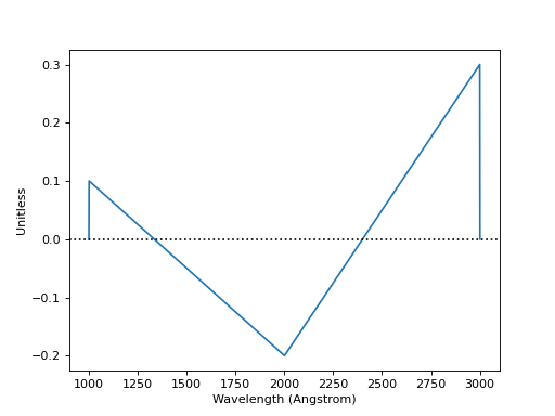
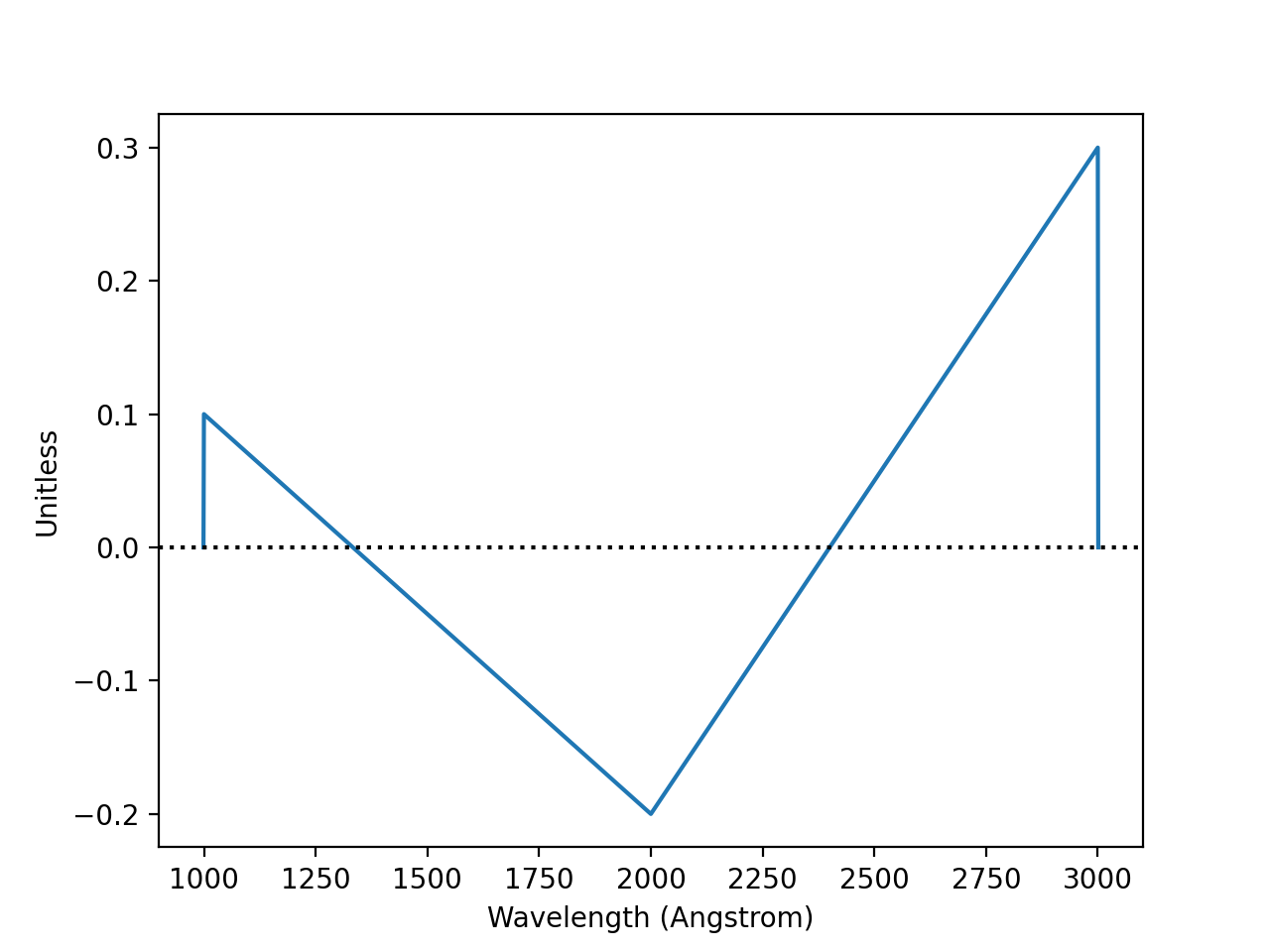
The example below creates and plots a bandpass from some given arrays. It also demonstrates that you can choose to keep negative throughput values (however unrealistic), if desired:
from synphot import SpectralElement
from synphot.models import Empirical1D
wave = [999, 1000, 2000, 3000, 3001]  # Angstrom
thru = [0, 0.1, -0.2, 0.3, 0]
bp = SpectralElement(
    Empirical1D, points=wave, lookup_table=thru, keep_neg=True)
bp.plot()
plt.axhline(0, color='k', ls=':')
(Source code, png, hires.png, pdf)

Box
A box-shaped bandpass is a rectangular window centered on a given wavelength with a given width. It is defined as:
where
\(f(x)\) is the throughput
\(x_{0}\) is the central wavelength
\(x\) is the wavelength array
\(w\) is the width of the box
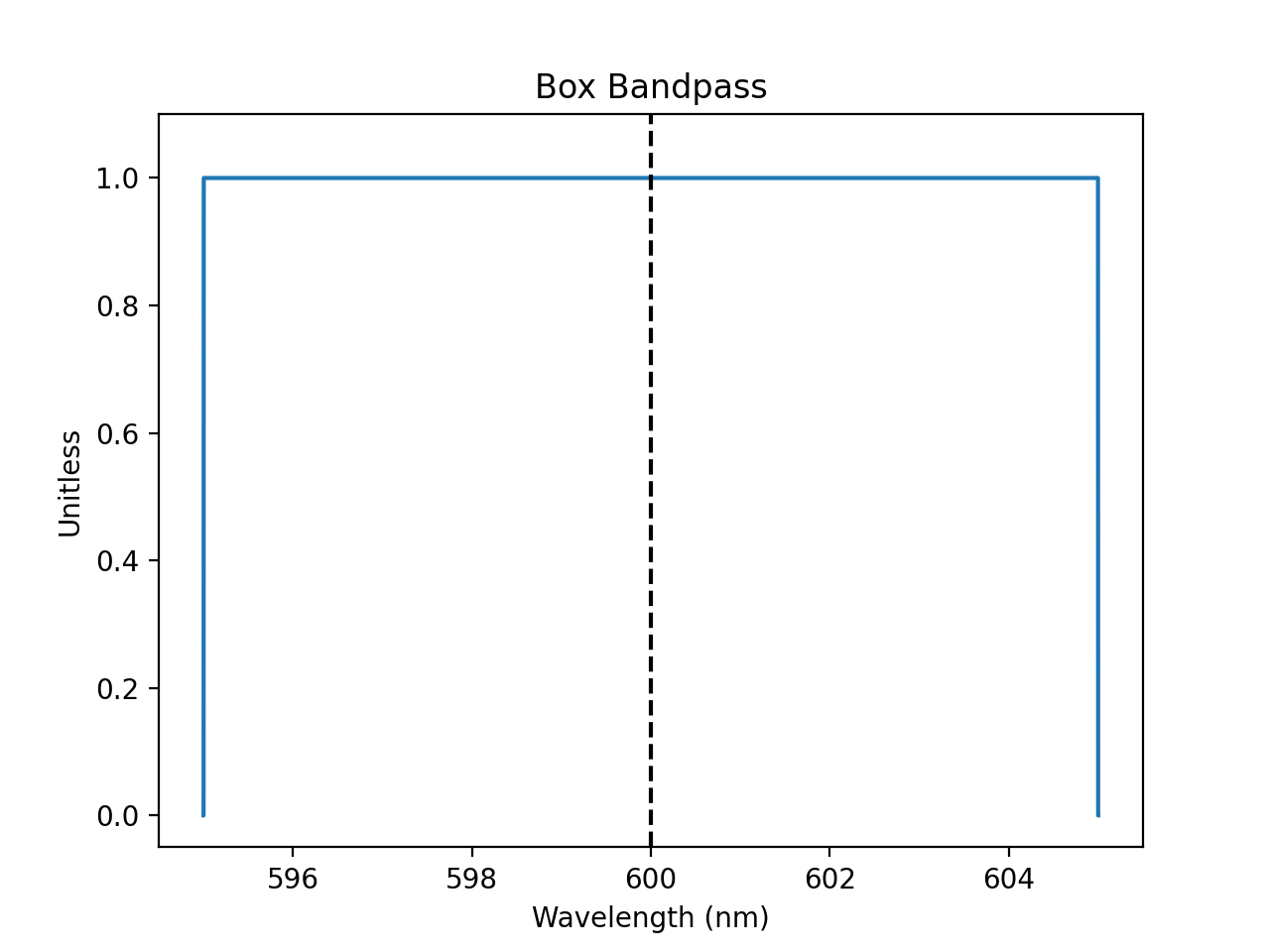
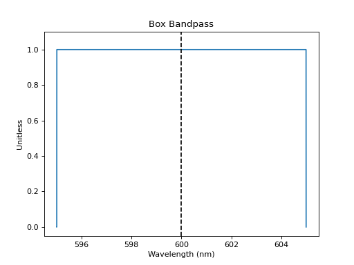
The example below creates and plots a box-shaped bandpass centered at 600 nm with a width of 10 nm:
import matplotlib.pyplot as plt
from astropy import units as u
from synphot import SpectralElement
from synphot.models import Box1D
bp = SpectralElement(Box1D, amplitude=1, x_0=600*u.nm, width=10*u.nm)
# Plot at user unit instead of internal unit
bp.plot(wavelengths=bp.waveset.to(u.nm), top=1.1, title='Box Bandpass')
plt.axvline(600, ls='--', color='k')
(Source code, png, hires.png, pdf)
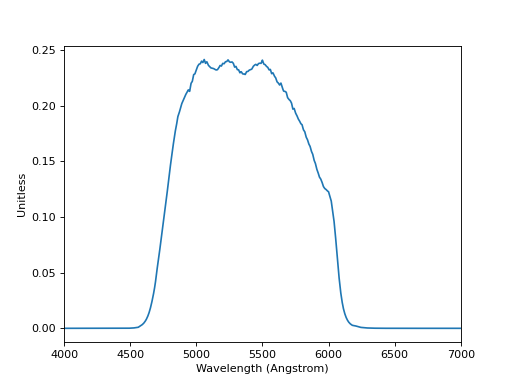
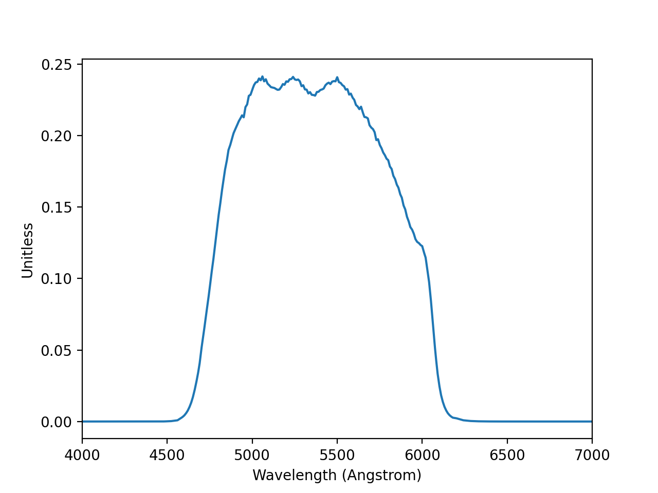
File
A bandpass can also be defined using a FITS or ASCII table containing columns of wavelength and throughput. See FITS Table Format and ASCII Table Format for details on how to create such tables.
The example below loads and plots a bandpass from FITS table in the software test data directory:
import os
from astropy.utils.data import get_pkg_data_filename
from synphot import SpectralElement
filename = get_pkg_data_filename(
    os.path.join('data', 'hst_acs_hrc_f555w.fits'),
    package='synphot.tests')
bp = SpectralElement.from_file(filename)
bp.plot(left=4000, right=7000)
(Source code, png, hires.png, pdf)

Filter
Pre-defined bandpass for some common filters are provided for convenience.
(See Installation and Setup for instructions on how to obtain the
data files.) They can be accessed via
from_filter() by passing in the
appropriate filter names:
'bessel_j'(Bessel J)'bessel_h'(Bessel H)'bessel_k'(Bessel K)'cousins_r'(Cousins R)'cousins_i'(Cousins I)'johnson_u'(Johnson U)'johnson_b'(Johnson B)'johnson_v'(Johnson V)'johnson_r'(Johnson R)'johnson_i'(Johnson I)'johnson_j'(Johnson J)'johnson_k'(Johnson K)
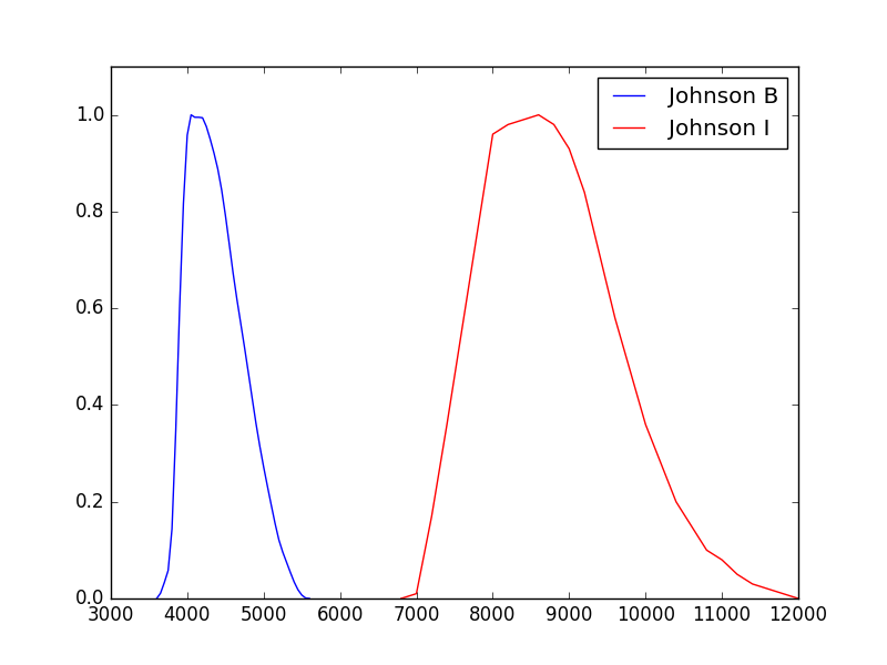
The example below loads and plots bandpasses from Johnson BI:
>>> import matplotlib.pyplot as plt
>>> from synphot import SpectralElement
>>> b = SpectralElement.from_filter('johnson_b')
>>> i = SpectralElement.from_filter('johnson_i')
>>> plt.plot(b.waveset, b(b.waveset), 'b', i.waveset, i(i.waveset), 'r')
>>> plt.ylim(0, 1.1)
>>> # Label comes from DESCRIP keyword from FITS header
>>> plt.legend([b.meta['header']['descrip'], i.meta['header']['descrip']])
For more extensive selection of filter systems, please use Synthetic Photometry for HST (stsynphot) and see its Non-HST Filter Systems.
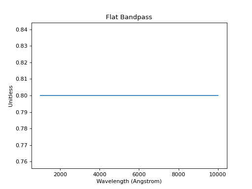
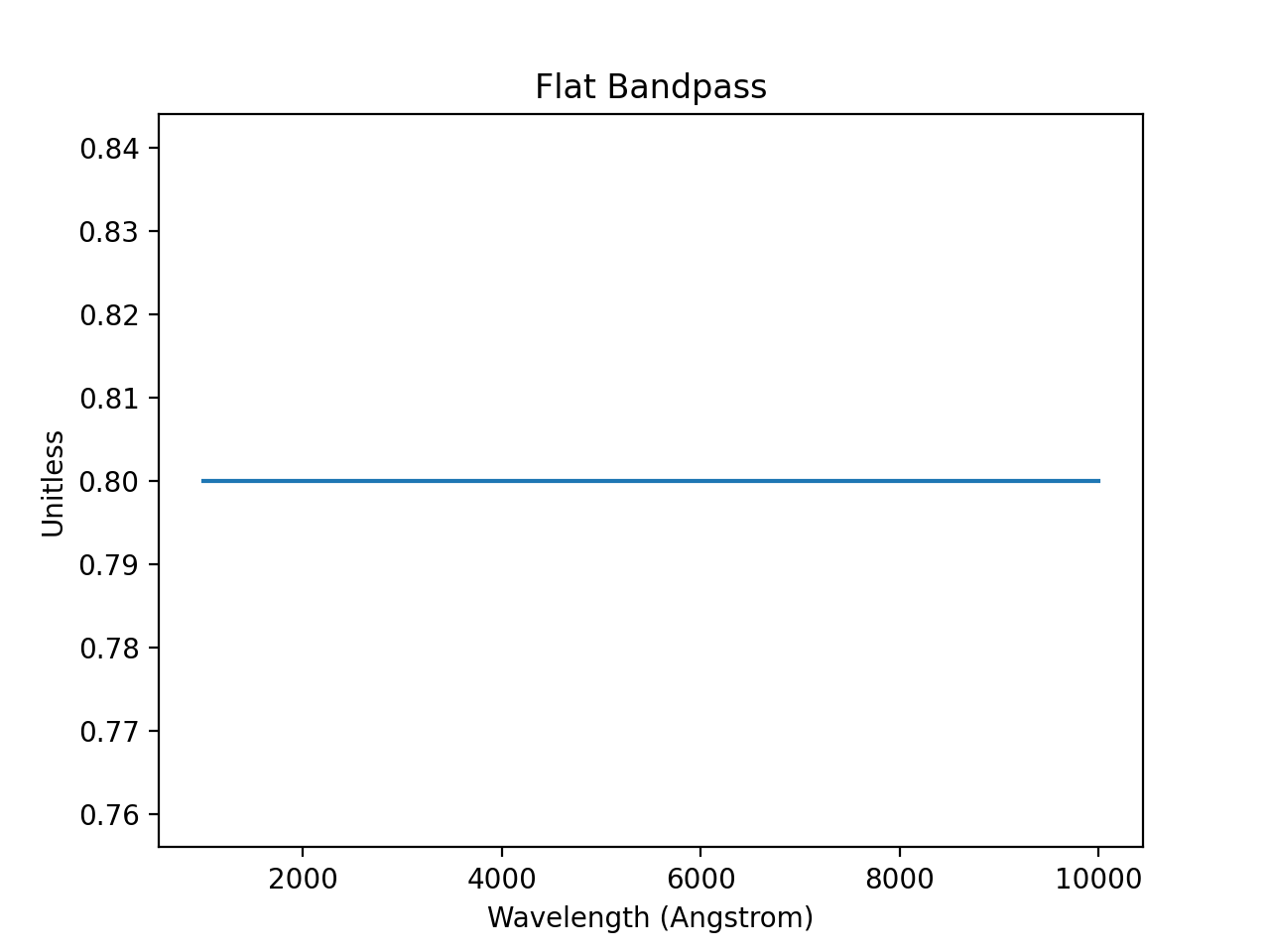
Flat
A flat (uniform) bandpass has a constant throughput at any wavelength value. It is defined as:
where
\(f(x)\) is the throughput
\(x\) is the wavelength array
\(A\) is the constant
The example below creates and plots a flat bandpass with its transmission set at 0.8:
from astropy.modeling.models import Const1D
from synphot import SpectralElement
bp = SpectralElement(Const1D, amplitude=0.8)
bp.plot([1000, 10000], title='Flat Bandpass')
(Source code, png, hires.png, pdf)

specutils
A bandpass can be constructed from and written to specutils.Spectrum1D
object. See specutils documentation for more
information on how to use Spectrum1D.
The example below writes a Box to a
Spectrum1D object:
>>> from astropy import units as u
>>> from synphot import SpectralElement
>>> from synphot.models import Box1D
>>> bp = SpectralElement(Box1D, amplitude=1, x_0=600*u.nm, width=10*u.nm)
>>> spec = bp.to_spectrum1d()
Meanwhile, this example reads in a bandpass from a
Spectrum1D object:
>>> from astropy import units as u
>>> from specutils import Spectrum1D
>>> from synphot import SpectralElement
>>> spec = Spectrum1D(spectral_axis=[100, 300]*u.nm,
...                   flux=[0.1, 0.8]*u.dimensionless_unscaled)
>>> bp = SpectralElement.from_spectrum1d(spec)