Tutorials
This page contains tutorials of specific synphot functionality not explicitly covered in other sections.
Emission Line
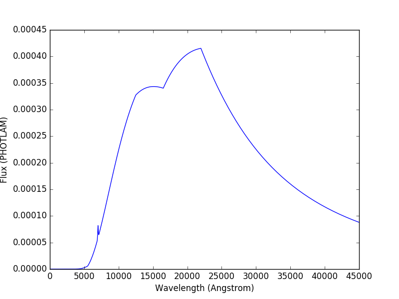
This tutorial is adapted from Exposure Time Calculator User’s Guide on a similar topic. In this tutorial, you will learn how to manipulate and superimpose an emission line to a continuum spectrum.
Create a continuum spectrum of a 5500 K blackbody with z=0.6:
>>> from synphot import SourceSpectrum
>>> from synphot.models import BlackBodyNorm1D
>>> bb = SourceSpectrum(BlackBodyNorm1D, temperature=5500, z=0.6)
Create a Gaussian emission line with 8E-14 FLAM total flux, FWHM of 100 Angstrom, and centered at 7000 Angstrom:
>>> from astropy import units as u
>>> from synphot import units
>>> from synphot.models import GaussianFlux1D
>>> em = SourceSpectrum(
...     GaussianFlux1D, total_flux=8e-14*u.erg/(u.cm**2 * u.s),
...     fwhm=100, mean=7000)
Add emission line to continuum spectrum:
>>> sp = bb + em
Apply extinction curve for LMC (average) with E(B-V)=1.3 to the composite spectrum:
>>> from synphot import ReddeningLaw
>>> ext = ReddeningLaw.from_extinction_model(
...     'lmcavg').extinction_curve(1.3)
>>> my_spec = sp * ext
Plot the result:
>>> my_spec.plot(right=45000)
Continuum-Normalized Spectrum
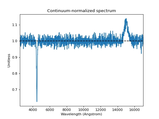
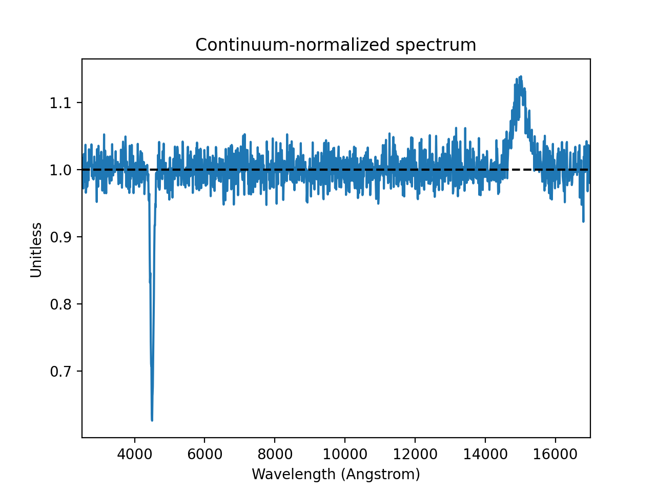
In this tutorial, you will learn how to create a composite spectrum with a noisy blackbody continuum, an emission line, and an absorption line. Then, you will divide it by a smooth continuum and plot the resultant continuum-normalized spectrum.
import matplotlib.pyplot as plt
import numpy as np
from astropy import units as u
from synphot import SourceSpectrum, BaseUnitlessSpectrum
from synphot.models import BlackBodyNorm1D, Empirical1D, GaussianFlux1D
np.random.seed(1234)  # For reproducibility
# Create the smooth continuum that is a 5000 K blackbody.
bb = SourceSpectrum(BlackBodyNorm1D, temperature=5000)
# Then, add random noise to it. Since synphot spectrum object cannot
# be multiplied with scalar array, this has to be done indirectly by
# applying the noise as a unitless spectrum.
wave = np.arange(100, 30001, 10)
nse = 1 + np.random.normal(size=wave.size, scale=0.02)
sp_nse = BaseUnitlessSpectrum(Empirical1D, points=wave, lookup_table=nse)
bb_noisy = bb * sp_nse
# Apply emission and absorption lines to the noisy continuum.
tf_unit = u.erg / (u.cm**2 * u.s)
g_em = SourceSpectrum(
    GaussianFlux1D, total_flux=2.65e-14*tf_unit, mean=15000, fwhm=500)
g_ab = SourceSpectrum(
    GaussianFlux1D, total_flux=6.62e-14*tf_unit, mean=4500, fwhm=100)
sp = bb_noisy + g_em - g_ab
# Divide the noisy spectrum with lines with the original smooth continuum
# to obtain the continuum-normalized spectrum.
ratio = sp / bb
with np.errstate(invalid='ignore'):
    ratio.plot(left=2500, right=17000,
               title='Continuum-normalized spectrum')
plt.axhline(1, ls='--', color='k')
(Source code, png, hires.png, pdf)

Using dust-extinction model
In this tutorial, you will learn how to apply an extinction curve using a model from the dust-extinction package:
>>> import numpy as np
>>> from astropy import units as u
>>> from dust_extinction.parameter_averages import CCM89
>>> from synphot import SourceSpectrum, ReddeningLaw
>>> from synphot.models import BlackBodyNorm1D
>>> ccm89_model = CCM89(Rv=3.1)
>>> wav = np.arange(0.1, 3, 0.001) * u.micron
>>> ebv = 0.1  # E(B-V)
>>> redlaw = ReddeningLaw(ccm89_model)
>>> extcurve = redlaw.extinction_curve(ebv, wavelengths=wav)
>>> bb = SourceSpectrum(BlackBodyNorm1D, temperature=5000 * u.K)
>>> bb.integrate()
<Quantity 9.31004028 ph / (s cm2)>
>>> sp = bb * extcurve
>>> sp.integrate()
<Quantity 8.27106961 ph / (s cm2)>
Fitting, Equivalent Width
In this tutorial, you will learn how to fit a Gaussian model to some real data and calculate its equivalent width. This is not handled by synphot but it is included here for those who are interested to see how fitting in IRAF SYNPHOT is done in Python. See Models and Fitting (astropy.modeling) for more information about fitting a model.
Read in the real data. If your own data has a different format, you need to adjust the example accordingly:
>>> from astropy.io import fits
>>> with fits.open('/path/to/combined_13330_G130M_v40_bin4.fits') as pf:
...     dat = pf[1].data
...     wave = dat.field('WAVELENGTH').flatten()  # Angstrom
...     flux = dat.field('FLUX').flatten()  # FLAM
For a good fit, only use data around the feature of interest. In this example, the feature is between 1202 and 1211 Angstrom:
>>> mask = (wave >= 1202) & (wave <= 1211)
>>> x = wave[mask]
>>> y = flux[mask]
Create a composite model with some initial parameters close to the desired result (usually sufficient to guess from looking at a plot of the data) and fit it using some fitter that is best for the data (sometimes, several iterations are required for a good fit):
>>> from astropy.modeling import models, fitting
>>> bg = models.Const1D(amplitude=3.5E-14)
>>> gs = models.Gaussian1D(amplitude=3.5E-14, mean=1206, stddev=1)
>>> init_model = bg - gs
>>> fitter = fitting.LevMarLSQFitter()
>>> fit_model = fitter(init_model, x, y)
>>> y_fit = fit_model(x)
>>> print(fit_model)
Model: CompoundModel...
Inputs: ('x',)
Outputs: ('y',)
Model set size: 1
Expression: [0] - [1]
Components:
    [0]: <Const1D(amplitude=3.5e-14)>

    [1]: <Gaussian1D(amplitude=3.5e-14, mean=1206.0, stddev=1.0)>
Parameters:
       amplitude_0       amplitude_1        mean_1       stddev_1
    ----------------- ----------------- ------------- -------------
    3.63064137361e-14 3.62623007738e-14 1206.27454371 0.23713207018
Plot the fitted model on top of input data:
>>> import matplotlib.pyplot as plt
>>> from matplotlib import ticker
>>> fig, ax = plt.subplots()
>>> ax.plot(x, y, 'b', x, y_fit, 'r')
>>> ax.get_xaxis().set_major_formatter(
...     ticker.FuncFormatter(ticker.FormatStrFormatter('%.0f')))
>>> ax.set_xlabel('Wavelength (Angstrom)')
>>> ax.set_ylabel('Flux (FLAM)')
>>> ax.legend(['Data', 'Fit'], loc='lower right')
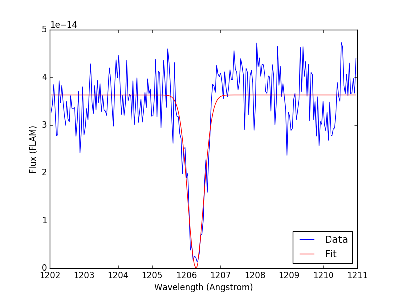
Calculate equivalent width using the fitted model:
>>> import math
>>> area = (math.sqrt(2 * math.pi) * fit_model.amplitude_1 *
...     fit_model.stddev_1)  # Area under curve
>>> height = fit_model.amplitude_0  # Continuum level
>>> print('EW = {:.4f} Angstrom'.format(area / height))
EW = 0.5937 Angstrom
Lyman-Alpha Extinction
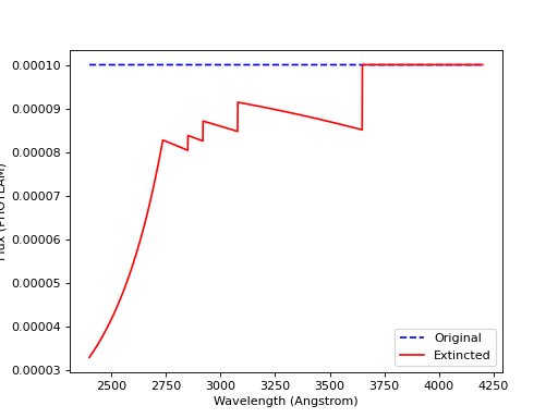
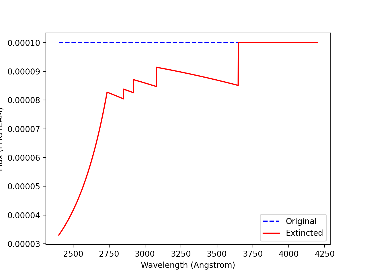
In this tutorial, you will learn how to apply extinction curve due to Lyman-alpha forest (Madau et al. 1995) to a source spectrum. For clarity, we will only use a flat source.
import matplotlib.pyplot as plt
from synphot import SourceSpectrum, etau_madau
from synphot.models import ConstFlux1D
# Create a flat source
sp = SourceSpectrum(ConstFlux1D, amplitude=1E-4)
# Apply extinction for a given redshift
z = 2
wave = range(2400, 4200)  # Angstrom
extcurve = etau_madau(wave, z)
sp_ext = sp * extcurve
# Compare the source with and without extinction
plt.plot(wave, sp(wave), 'b--', wave, sp_ext(wave), 'r')
plt.xlabel('Wavelength (Angstrom)')
plt.ylabel('Flux (PHOTLAM)')
plt.legend(['Original', 'Extincted'], loc='lower right')
(Source code, png, hires.png, pdf)

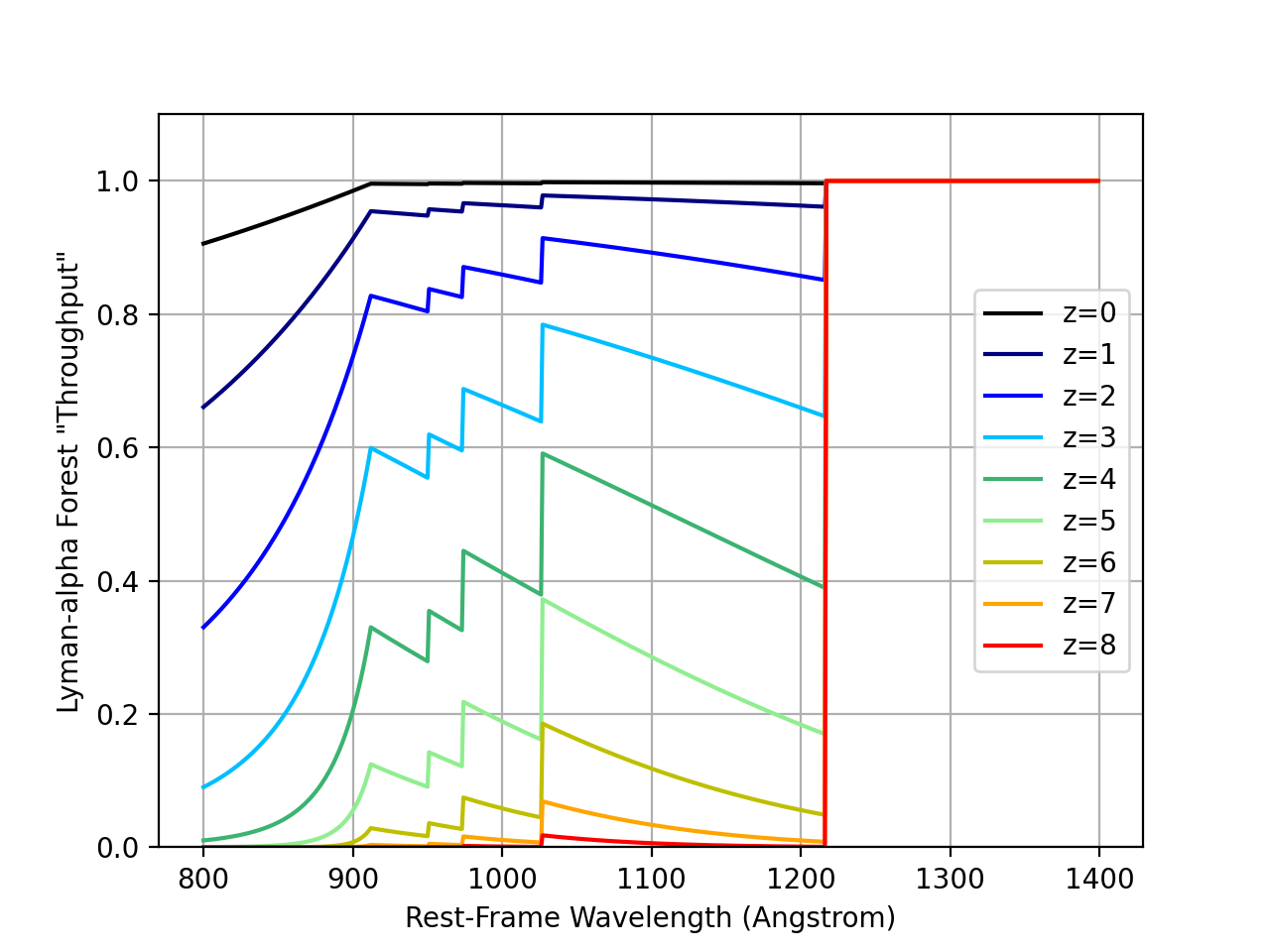
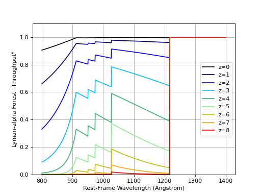
The chart below illustrates the Madau 1995 extinction curves for different redshift values. For clarity, they are plotted against rest wavelength, not the redshifted wavelength:
import matplotlib.pyplot as plt
import numpy as np
from synphot import etau_madau
w_rest = np.arange(800, 1400)
lc = ['k', 'navy', 'b', 'deepskyblue', 'mediumseagreen',
      'lightgreen', 'y', 'orange', 'r']
for z in range(0, 9):
    wave = w_rest * (1 + z)
    extcurve = etau_madau(wave, z)
    plt.plot(w_rest, extcurve(wave), color=lc[z], label='z={}'.format(z))
plt.ylim(0, 1.1)
plt.xlabel('Rest-Frame Wavelength (Angstrom)')
plt.ylabel('Lyman-alpha Forest "Throughput"')
plt.legend(loc='center right')
plt.grid()
(Source code, png, hires.png, pdf)
Setting Area for XMM-OM
Some telescopes (e.g., XMM-OM by ESA) provide throughput curves with effective
area information embedded in them already. In the case of XMM-OM, its
throughput curves are in effective_area * 100 meter squared, for which we
would divide each throughput curve loaded into SpectralElement by 100.
We also would set the primary area, when it is needed, as follows:
>>> from astropy import units as u
>>> area = 1 * (u.m * u.m)