Observation
Observation is a special type of
Source Spectrum,
where the source is convolved with a Bandpass; i.e., a photon has
already passed through the telescope optics. It is usually the end-point of a
chain of spectral manipulation. Unlike a regular source spectrum, there is only
one way to create an observation; i.e., by passing in source and bandpass
objects into its constructor. Operations that do not make sense in the context
of an observation (e.g., redshifting, tapering, addition, and subtraction) are
disabled.
An observation also understands detector binning. By default, the bins are
assumed to be the same as the waveset of the input bandpass. However,
this is not always true, particularly for “obsmode” in stsynphot. In those
cases, the bandpass has an extra binset attribute (wavelength values for
bin centers) that must be passed into an observation’s constructor, as shown
below:
>>> import stsynphot as stsyn
>>> from astropy import units as u
>>> from synphot import Observation, SourceSpectrum
>>> from synphot.models import GaussianFlux1D
>>> sp = SourceSpectrum(GaussianFlux1D, amplitude=1*u.Jy,
...                     mean=6000*u.AA, fwhm=100*u.AA)
>>> bp = stsyn.band('acs,hrc,f555w')
>>> obs = Observation(sp, bp, binset=bp.binset)
It has these main general components:
spectrum, the input source spectrumbandpass, the input bandpassmodel, the underlying Astropy composite modelwaveset, the wavelength set for “native” samplingwaverange, the range (inclusive) covered bywavesetmeta, metadata associated with the observationwarnings, special metadata to highlight any warning
It also has these components related to binning:
binset, center of the wavelength binsbin_edges, edges of the wavelength binsbinflux, binned flux computed by integrating the “native” flux over the width of each bin
To evaluate its flux at a given wavelength (not binned), use its
__call__() method as you would with any Astropy model
(except that the method also takes additional keywords like flux_unit
for flux conversion). To get binned flux values, use
sample_binned(), where you must provide
the exact bin center(s):
>>> obs(6000.5)  # Native (not binned) sampling; Angstrom
<Quantity 0.03080553 PHOTLAM>
>>> obs.sample_binned([6000, 6001])  # Binned flux in given centers
<Quantity [0.03084873, 0.0307453 ] PHOTLAM>
To calculate bin properties such as covered wavelength or pixel ranges,
you can use its binned_waverange() and
binned_pixelrange() as follows:
>>> # Wavelength range covered by 10 pixels centered at 5500 Angstrom
>>> obs.binned_waverange(5500, 10)
<Quantity [5495.5, 5505.5] Angstrom>
>>> # Pixel range covered by above wavelength range
>>> obs.binned_pixelrange([5495.5, 5505.5])
10
In addition, it has unique properties such as Effective Stimulus and Effective Wavelength, which can be calculated in a way that is consistent with ASTROLIB PYSYNPHOT:
>>> # Effective stimulus in FLAM
>>> obs.effstim(flux_unit='flam')
<Quantity 4.12569567e-14 FLAM>
>>> # Effective wavelength for binned sampling in FLAM
>>> obs.effective_wavelength()
<Quantity 5991.99794956 Angstrom>
>>> # Repeat for "native" sampling
>>> obs.effective_wavelength(binned=False)
<Quantity 5991.99798818 Angstrom>
countrate() is probably the most often
used method for an observation.
It computes the total counts (a special case of effective stimulus)
of a source spectrum, integrated over the bandpass with
some binning. By default, it uses binset, which should be defined such that
one wavelength bin corresponds to one detector pixel:
>>> area = 45238.93416  # HST, in cm^2
>>> obs.countrate(area)
<Quantity 137190.19332899 ct / s>
Note
If flux values contain NaNs, countrate() will raise SynphotError.
An observation can be converted to a regular source spectrum containing
only the wavelength set and sampled flux (binned by default) by using its
as_spectrum() method.
This is useful when you wish to access functionalities that are not directly
available to an observation (e.g., tapering or saving to a file).
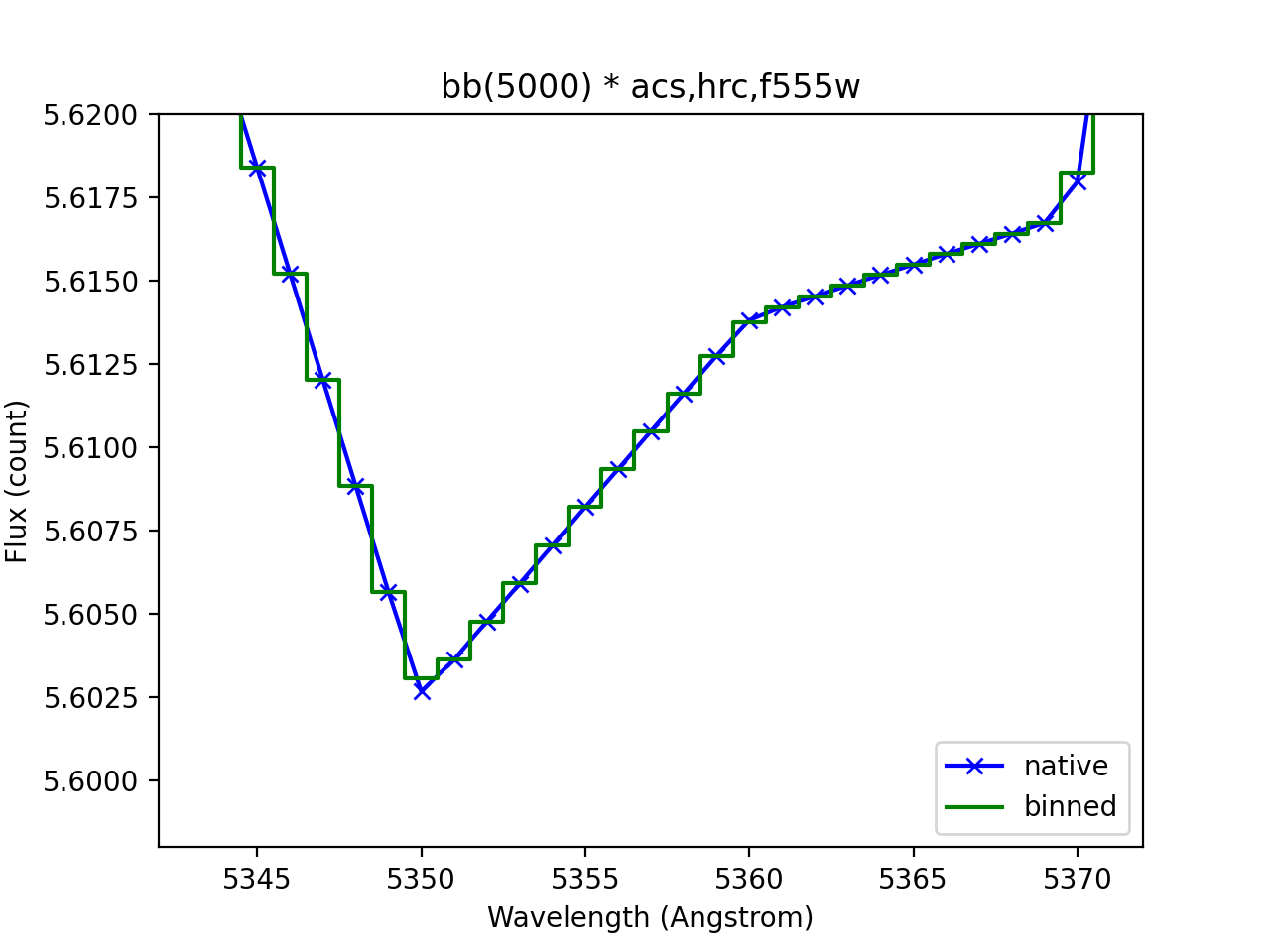
To accurately represent binned flux visually, especially in a unit like count
that is very sensitive to bin size, it is recommended to plot the data as a
histogram using binset as mid-points, as shown below:
import os
import matplotlib.pyplot as plt
from astropy.utils.data import get_pkg_data_filename
from synphot import Observation, SourceSpectrum, SpectralElement, units
from synphot.models import BlackBodyNorm1D
# Construct blackbody source
sp = SourceSpectrum(BlackBodyNorm1D, temperature=5000)
# Simulate an instrument bandpass with custom binning
bp = SpectralElement.from_file(get_pkg_data_filename(
    os.path.join('data', 'hst_acs_hrc_f555w.fits'),
    package='synphot.tests'))
binset = range(1000, 11001)
# Build the observation and get binned flux in count
obs = Observation(sp, bp, binset=binset)
area = 45238.93416 * units.AREA  # HST
binflux = obs.sample_binned(flux_unit='count', area=area)
# Sample the "native" flux for comparison
flux = obs(obs.binset, flux_unit='count', area=area)
# Plot with zoom to see native vs binned
plt.plot(obs.binset, flux, 'bx-', label='native')
plt.plot(obs.binset, binflux, 'g-', drawstyle='steps-mid', label='binned')
plt.xlim(5342, 5372)
plt.ylim(5.598, 5.62)
plt.xlabel('Wavelength (Angstrom)')
plt.ylabel('Flux (count)')
plt.title('bb(5000) * acs,hrc,f555w')
plt.legend(loc='lower right', numpoints=1)
(Source code, png, hires.png, pdf)

specutils
A specutils.Spectrum1D object can be passed directly into
Observation as a source spectrum. For example:
>>> from specutils import Spectrum1D
>>> spec = Spectrum1D(spectral_axis=[499, 500, 600, 601]*u.nm,
...                   flux=[0, 0.1, 0.8, 0]*u.nJy)
>>> obs = Observation(spec, bp, binset=binset)
>>> obs.effstim(u.ABmag)
<Magnitude 32.70048821 mag(AB)>