Synthetic Photometry (synphot)
Introduction
synphot simulates photometric data and spectra, observed or otherwise. You can incorporate your own filters, spectra, and data. You can also use a pre-defined standard star (Vega), bandpass, or extinction law. Furthermore, it allows you to:
Construct complicated composite spectra using different models.
Simulate observations.
Compute photometric properties such as count rate, effective wavelength, and effective stimulus.
Manipulate a spectrum; e.g., applying redshift or normalize it to a given flux value in a given bandpass.
Sample a spectrum at given wavelengths.
Plot a quick-view of a spectrum.
Perform repetitive operations such as simulating the observations of multiple type of sources through multiple bandpasses.
This package covers the general functionalities not related to any particular observatory. If you use HST, you might also be interested in stsynphot (https://github.com/spacetelescope/stsynphot_refactor), which covers synthetic photometry for the telescope(s).
If you use synphot in your work, please see CITATION for details on how to cite it in your publications.
If you have questions or concerns regarding the software, please open an issue at https://github.com/spacetelescope/synphot_refactor/issues (if not already reported) or contact STScI Help Desk.
Installation and Setup
synphot works for Python 3.10 or later only. It requires the following packages:
numpy
astropy
scipy
matplotlib (optional for plotting)
specutils (optional)
You can install synphot using one of the following ways:
From the
conda-forgechannel:conda install synphot -c conda-forge
From standalone release:
pip install synphot
From nightly wheel uploads (pre-built
devversion):pip install -i https://pypi.anaconda.org/stsci/simple synphot -U --pre
From source (example shown is for the
devversion):git clone https://github.com/spacetelescope/synphot_refactor.git cd synphot_refactor pip install .
To use the pre-defined standard star, extinction laws, and bandpasses, it is
recommended for non-internal STScI users to download the necessary data files to
a local directory so you can avoid connecting directly to STScI HTTP service,
which is slower and might not be available all the time. To download the files
via HTTP, create a local directory where you plan to store the data files
(e.g., /my/local/dir/trds) and run the following:
>>> from synphot.utils import download_data
>>> file_list = download_data('/my/local/dir/trds')
With astropy, you can generate a
$HOME/.astropy/config/synphot.cfg file like this (otherwise, you can
manually create one from synphot’s Default Configuration File):
>>> from astropy.config import generate_config
>>> generate_config(pkgname='synphot')
Then, you can modify it to your needs; Uncomment and replace every instance of
file prefix with /my/local/dir/trds so that synphot knows where to
look for these files.
On the contrary, if you wish to rely solely on Astropy caching mechanism,
you can use download_data(None), but make sure that you do not
modify your default $HOME/.astropy/config/synphot.cfg file. Otherwise,
synphot will try to use what is in synphot.cfg instead.
Note
synphot data files are a minimal subset of those required by stsynphot. If you plan to use the latter anyway, please also read the instructions in its documentation.
If you have your own version of the data files that you wish to use, you can
modify synphot.cfg to point to your own copies without having to download
using the function above. However, before you do so, make sure that your own
file(s) can be read in successfully with
read_fits_spec().
For example, if you want to use your own Johnson V throughput file, you
can modify this line in your $HOME/.astropy/config/synphot.cfg file:
johnson_v_file = /my/other/dir/my_johnson_v.fits
Alternately, you can also take advantage of Configuration System (astropy.config)
to manage synphot data files. This example below overwrites the
Johnson V throughput file setting for the entire Python session
(this supersedes what is set in synphot.cfg above):
>>> from synphot.config import conf
>>> conf.johnson_v_file = '/my/local/dir/trds/comp/nonhst/johnson_v_004_syn.fits'
>>> print(conf.johnson_v_file)
/my/local/dir/trds/comp/nonhst/johnson_v_004_syn.fits
Using the configuration system, you can also temporarily use a different Johnson V throughput file:
>>> with conf.set_temp('johnson_v_file', '/my/other/dir/my_johnson_v.fits'):
...     print(conf.johnson_v_file)
/my/other/dir/my_johnson_v.fits
>>> print(conf.johnson_v_file)
/my/local/dir/trds/comp/nonhst/johnson_v_004_syn.fits
Getting Started
This section only contains minimal examples showing how to use this package. For detailed documentation, see Using synphot.
In the examples below, you will notice that most models are from
synphot.models, not astropy.modeling.models, because the models in
synphot have extra things like sampleset that are not (yet) available
in Astropy. Despite this, some models like
Const1D does not need the extra things to
work, so they can be used directly. When in doubt, see if a model is in
synphot.models first before using Astropy’s.
>>> from astropy import units as u
>>> from synphot import units, SourceSpectrum
>>> from synphot.models import BlackBodyNorm1D, GaussianFlux1D
Create a Gaussian absorption line with the given amplitude centered at 4000 Angstrom with a sigma of 20 Angstrom:
>>> g_abs = SourceSpectrum(GaussianFlux1D, amplitude=1*u.mJy,
...                        mean=4000, stddev=20)
Create a Gaussian emission line with the given total flux centered at 3000 Angstrom with FWHM of 100 Angstrom:
>>> g_em = SourceSpectrum(GaussianFlux1D,
...                       total_flux=3.5e-13*u.erg/(u.cm**2 * u.s),
...                       mean=3000, fwhm=100)
Create a blackbody source spectrum with a temperature of 6000 K:
>>> bb = SourceSpectrum(BlackBodyNorm1D, temperature=6000)
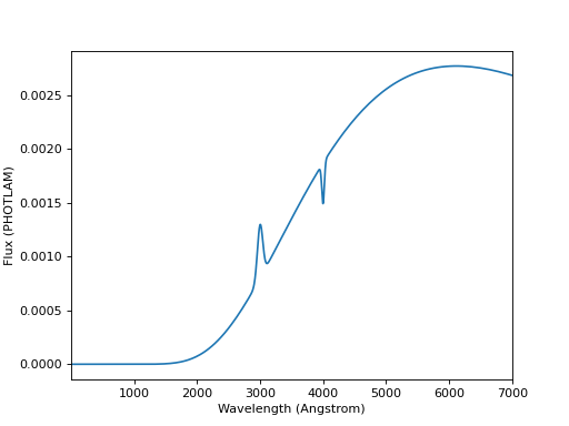
Combine the above components to create a source spectrum that is twice the original blackbody flux with the Gaussian emission and absorption lines:
>>> sp = 2 * bb + g_em - g_abs
Plot the spectrum, zooming in on the line features:
>>> sp.plot(left=1, right=7000)
(Source code, png, hires.png, pdf)

Sample the spectrum at 0.3 micron:
>>> sp(0.3 * u.micron)
<Quantity 0.00129536 PHOTLAM>
Or sample the same thing but in a different flux unit:
>>> sp(0.3 * u.micron, flux_unit=units.FLAM)
<Quantity 8.57718043e-15 FLAM>
Sample the spectrum at its native wavelength set:
>>> sp(sp.waveset)
<Quantity [0.00000000e+00, 0.00000000e+00, 0.00000000e+00, ...,
           4.47483872e-05, 4.34265235e-05, 4.21423946e-05] PHOTLAM>
Models that built the spectrum:
>>> print(sp)
SourceSpectrum at z=0.0
Model: CompoundModel...
Inputs: ('x',)
Outputs: ('y',)
Model set size: 1
Expression: ([0] | [1]) + [2] - [3]
Components:
    [0]: <BlackBodyNorm1D(...)>

    [1]: <Scale(...)>

    [2]: <GaussianFlux1D(...)>

    [3]: <GaussianFlux1D(...)>
Parameters:
    ...
Redshift the source spectrum by \(z = 0.2\):
>>> sp.z = 0.2
Create a box-shaped bandpass centered at 4000 Angstrom with a width of 2000 Angstrom:
>>> from synphot import SpectralElement
>>> from synphot.models import Box1D
>>> bp = SpectralElement(Box1D, amplitude=1, x_0=4000, width=2000)
Normalize the source spectrum to 1 Jy in a given box bandpass and integrate it:
>>> sp_rn = sp.normalize(1 * u.Jy, band=bp)
>>> sp_rn.integrate()
<Quantity 12540.4613615 ph / (s cm2)>
Create an observation by passing the redshifted and normalized source spectrum through the box bandpass:
>>> from synphot import Observation
>>> obs = Observation(sp_rn, bp)
Calculate the count rate of the observation above for an 2-meter telescope:
>>> import numpy as np
>>> area = np.pi * (1 * u.m) ** 2
>>> area
<Quantity 3.14159265 m2>
>>> obs.countrate(area=area)
<Quantity 24219649.46880912 ct / s>
Using synphot
A Brief History
A brief history: First, there was STSDAS SYNPHOT (IRAF). Then, there was ASTROLIB PYSYNPHOT (Lim et al. 2015), which aimed at replacing STSDAS SYNPHOT using Python. In order to take advantage of Models and Fitting (astropy.modeling) and Units and Quantities (astropy.units) and to repurpose the functionality for a wider audience (other than HST users), it was refactored again and separated into synphot and stsynphot (see Synthetic Photometry (synphot)).
API
synphot.binning Module
Utilities related to wavelength bin calculations.
Functions
|
Calculate the edges of wavelength bins given the centers. |
|
Calculate the widths of wavelengths bins given their edges. |
|
Calculate the centers of wavelengths bins given their edges. |
|
Calculate the wavelength range covered by the given number of pixels centered on the given central wavelength of the given bins. |
|
Calculate the number of pixels within the given wavelength range and the given bins. |
Also imports this C-extension to local namespace:
synphot.blackbody Module
Model and functions related to blackbody radiation.
Note
This was astropy.modeling.blackbody module that was
deprecated in astropy 4.0. The content is copied here
so we can still use it without deprecation warning.
Eventually, when we can fully pass in unit handling directly
to Astropy models, we can remove this module. See
https://github.com/astropy/astropy/pull/9282 and
https://github.com/spacetelescope/synphot_refactor/pull/224 .
Functions
|
Calculate blackbody flux per steradian, \(B_{\nu}(T)\). |
|
Like |
Classes
|
One dimensional blackbody model. |
synphot.config Module
Synphot configurable items.
The default configuration heavily depends on STScI TRDS structure
but it can be easily re-configured as the user wishes via
astropy.config.
synphot.exceptions Module
Exceptions specific to synthetic photometry.
Classes
Base class for synphot exceptions. |
|
|
Exceptions to do with table access. |
|
Duplicate wavelengths are not allowed in table. |
|
Zero wavelengths are not allowed in table. |
|
Unsorted wavelengths are not allowed in table. |
Exceptions to do with overlap checking. |
|
Partial overlap is not allowed. |
|
Disjoint data is not allowed. |
|
Exceptions for undefined bin set. |
|
Two sources in composite spectrum are not compatible. |
|
Exceptions for interpolation. |
|
Exceptions for extrapolation. |
Class Inheritance Diagram
synphot.filter_parameterization Package
This subpackage handles filter parameterization.
The algorithms in this subpackage were originally developed by Brett Morris as part of the tynt package.
Functions
|
Similar to |
|
Reconstruct a filter from given FFT parameters. |
|
Calculate filter parameters using FFT. |
|
Run |
synphot.models Module
Spectrum models not in astropy.modeling.
Functions
|
Get optimal wavelengths for sampling a given model. |
|
Get metadata for a given model. |
Classes
|
Create a blackbody spectrum model with given temperature. |
|
Create a normalized blackbody spectrum with given temperature. |
|
Same as |
|
One dimensional constant flux model. |
|
Empirical (sampled) spectrum or bandpass model. |
|
Same as |
|
Same as |
|
Same as |
|
Same as |
|
This is the deprecated name for |
|
Same as |
|
One dimensional power law model with proper flux handling. |
|
Same as |
Class Inheritance Diagram
synphot.observation Module
This module defines an observed spectrum, i.e., a source spectrum that has gone through a bandpass.
Classes
|
This is an observed spectrum, where a source spectrum has gone through a bandpass. |
Class Inheritance Diagram
synphot.reddening Module
This module defines reddening laws and extinction curves.
Functions
|
Madau 1995 extinction for a galaxy at given redshift. |
Classes
|
Model to handle extinction curve. |
|
Class to handle reddening law. |
|
Class to handle extinction curve. |
Class Inheritance Diagram
synphot.specio Module
This modules handles synthetic photometry data formats.
Functions
|
Read FITS or ASCII spectrum from a remote location. |
|
Read FITS or ASCII spectrum. |
|
Read ASCII spectrum. |
|
Read FITS spectrum. |
|
Write FITS spectrum. |
synphot.spectrum Module
This module defines the different types of spectra.
Functions
|
Convenience function to load a default Vega spectrum that is used throughout |
Classes
|
Base class to handle spectrum or bandpass. |
|
Base class to handle spectrum with flux unit like source spectrum and observation. |
|
Class to handle source spectrum. |
|
Base class to handle unitless spectrum like bandpass, reddening, etc. |
|
Class to handle instrument filter bandpass. |
Variables
Default Vega spectrum. |
synphot.thermal Module
This module defines thermal spectra.
Classes
|
Class to handle spectral element with associated thermal properties. |
Class Inheritance Diagram
synphot.units Module
This module handles photometry units that are not in astropy.units.
Functions
|
Flux equivalencies between PHOTLAM and VEGAMAG. |
|
Flux equivalencies between PHOTLAM and count/OBMAG. |
|
Perform conversion for supported flux units. |
|
Validate unit. |
|
Like |
|
Validate quantity (value and unit). |
synphot.utils Module
Synthetic photometry utility functions.
Functions
|
Check overlap between two arrays. |
|
Check integrated flux for invalid values. |
|
Check wavelengths for |
|
Generate wavelength array to be used for spectrum sampling. |
|
Return the union of the two sets of wavelengths using |
|
Download |
References
Calzetti, D., Armus, L., Bohlin, R. C., Kinney, A. L., Koornneef, J., & Storchi-Bergmann, T. 2000, ApJ, 533, 682
Cardelli, J. A., Clayton, G. C., & Mathis, J. S. 1989, ApJ, 345, 245
Gordon, K. D., Clayton, G. C., Misselt, K. A., Landolt, A. U., & Wolff, M. J. 2003, ApJ, 594, 279
Horne, K. 1988, in New Directions in Spectophotometry: A Meeting Held in Las Vegas, NV, March 28-30, Application of Synthetic Photometry Techniques to Space Telescope Calibration, ed. A. G. Davis Philip, D. S. Hayes, & S. J. Adelman (Schenectady, NY: L. Davis Press), 145
Koornneef, J., Bohlin, R., Buser, R., Horne, K., & Turnshek, D. 1986, Highlights Astron., 7, 833
Laidler, V., et al. 2008, Synphot Data User’s Guide, Version 1.2 (Baltimore, MD: STScI)
Lim, P. L., Diaz, R. I., & Laidler, V. 2015, PySynphot User’s Guide (Baltimore, MD: STScI), https://pysynphot.readthedocs.io/en/latest/
Madau, P., et al. 1995, ApJ, 441, 18
Oke, J. B., 1974, ApJS, 27, 21
Rybicki, G. B., & Lightman, A. P. 1979, Radiative Processes in Astrophysics (New York, NY: Wiley)
Schneider, D. P., Gunn, J. E., & Hoessel J. G. 1983, ApJ, 264, 337