Source Spectrum

A source spectrum is used to represent astronomical sources, such as stars and galaxies. An Observation is a special case of a source spectrum that is convolved with a Bandpass.

A source spectrum can be constructed by one of the following methods:

• Load a supported FITS file or ASCII file with from_file().

• Use the pre-defined Vega spectrum, which is also used to define VEGAMAG, with from_vega().

• Pass a supported model along with the keywords needed to define it into a SourceSpectrum object.

• Create a thermal source spectrum with thermal_source().

• Build a composite source using Spectrum Arithmetic. (Also see example in Getting Started.)

• Build an empirical source using specutils.

It has these main components:

• z, the redshift applied, if any

• z_type that indicates whether redshift also conserves flux or not

• model, the underlying Astropy model

• waveset, the wavelength set for optimal sampling

• waverange, the range (inclusive) covered by waveset

• meta, metadata associated with the spectrum

• warnings, special metadata to highlight any warning

To evaluate its flux at a given wavelength, use its __call__() method as you would with any Astropy model (except that the method also takes additional keywords like flux_unit for flux conversion):

>>> from synphot import SourceSpectrum, units
>>> from synphot.models import ConstFlux1D
>>> sp = SourceSpectrum(ConstFlux1D, amplitude=1)  # PHOTLAM
>>> wave = [1000, 10000]  # Angstrom
>>> sp(wave)  
<Quantity [1., 1.] PHOTLAM>
>>> sp(wave, flux_unit=units.FNU)  
<Quantity [6.62607015e-24, 6.62607015e-23] FNU>
>>> area = 45238.93416 * units.AREA  # HST
>>> sp(wave, flux_unit=units.OBMAG, area=area)  
<Magnitude [-21.52438718,-21.52438718] mag(OB)>

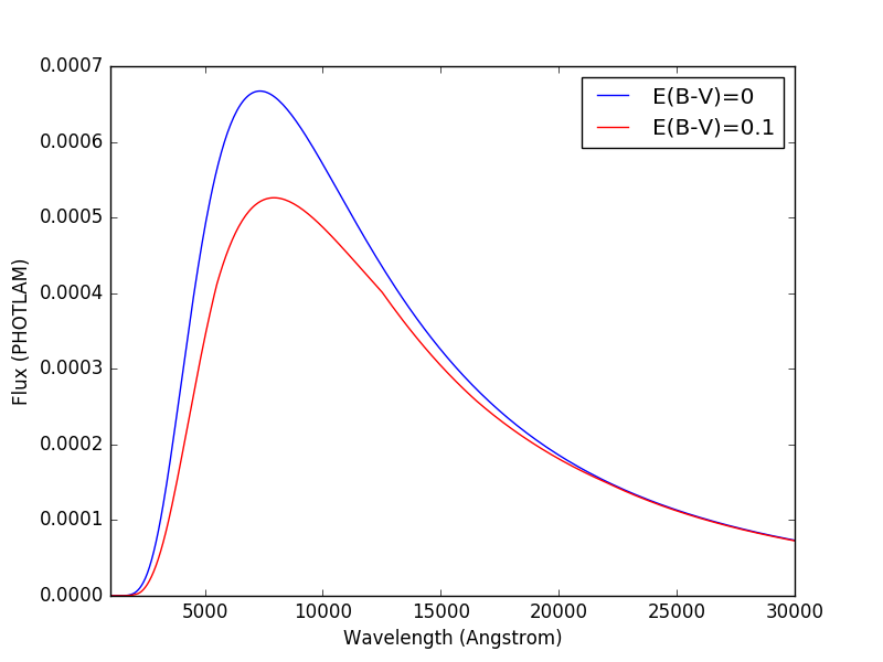
To apply (or remove) the effects of interstellar reddening on a source spectrum, use from_extinction_model() to provide a reddening model name (see table below; not to be confused with Astropy model) and then extinction_curve() to create the extinction curve with a given \(E(B-V)\) value (negative value effectively de-reddens the spectrum), and then multiply it to the source:

>>> import matplotlib.pyplot as plt  
>>> from synphot import SourceSpectrum, ReddeningLaw
>>> from synphot.models import BlackBodyNorm1D
>>> em = SourceSpectrum(BlackBodyNorm1D, temperature=5000)
>>> ext = ReddeningLaw.from_extinction_model(
...     'lmcavg').extinction_curve(0.1)  
>>> sp = em * ext  
>>> wave = em.waveset
>>> plt.plot(wave, em(wave), 'b', wave, sp(wave), 'r')  
>>> plt.xlim(1000, 30000)  
>>> plt.xlabel('Wavelength (Angstrom)')  
>>> plt.ylabel('Flux (PHOTLAM)')  
>>> plt.legend(['E(B-V)=0', 'E(B-V)=0.1'], loc='upper right')  

Name	Description	Reference
mwavg	Milky Way Diffuse, R(V)=3.1	Cardelli et al. (1989)
mwdense	Milky Way Dense, R(V)=5.0
mwrv21	Milky Way CCM, R(V)=2.1
mwrv40	Milky Way CCM, R(V)=4.0
lmc30dor	LMC Supershell, R(V)=2.76	Gordon et al. (2003)
lmcavg	LMC Average, R(V)=3.41
smcbar	SMC Bar, R(V)=2.74
xgalsb	Starburst, R(V)=4.0 (attenuation law)	Calzetti et al. (2000)

For extinction due to Lyman-alpha forest, see Lyman-Alpha Extinction tutorial. To use a model from the dust-extinction package, see Using dust-extinction model.

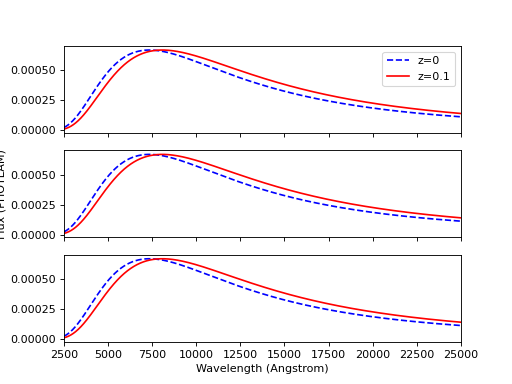
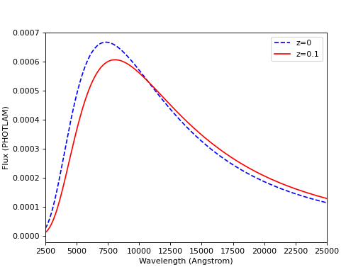
You can redshift a source spectrum in several ways (shown in example below), either by setting its z attribute or passing in a z keyword during initialization. To blueshift, you may use the same attribute/keyword but set its value to \(\frac{1}{1 + z} - 1\) instead. By default, only the wavelength values are shifted, not the flux (i.e., total flux is not preserved):

import matplotlib.pyplot as plt
from synphot import SourceSpectrum
from synphot.models import BlackBodyNorm1D
fig, ax = plt.subplots(3, sharex=True)
# Create a source at rest wavelength and sample it because it will
# be modified in-place below
sp_rest = SourceSpectrum(BlackBodyNorm1D, temperature=5000)
wave = range(2500, 25000, 10)
flux = sp_rest(wave)
# Redshift the original source as a new spectrum
sp_z1 = SourceSpectrum(sp_rest.model, z=0.1)
ax[0].plot(wave, flux, 'b--', wave, sp_z1(wave), 'r')
# Redshift the original source in-place
sp_rest.z = 0.1
ax[1].plot(wave, flux, 'b--', wave, sp_rest(wave), 'r')
# Create a redshifted source from scratch
sp_z2 = SourceSpectrum(BlackBodyNorm1D, temperature=5000, z=0.1)
ax[2].plot(wave, flux, 'b--', wave, sp_z2(wave), 'r')
# Extra plot commands
ax[2].set_xlim(2500, 25000)
ax[2].set_xlabel('Wavelength (Angstrom)')
ax[1].set_ylabel('Flux (PHOTLAM)')
ax[0].legend(['z=0', 'z=0.1'], loc='upper right')

(Source code, png, hires.png, pdf)

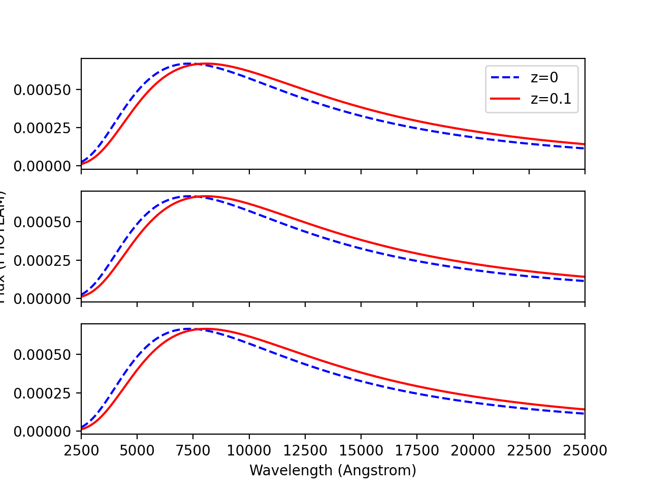
You can also redshift while preserving flux by setting z_type to 'conserve_flux':

import matplotlib.pyplot as plt
from synphot import SourceSpectrum
from synphot.models import BlackBodyNorm1D
# Create a source at rest wavelength
sp_rest = SourceSpectrum(BlackBodyNorm1D, temperature=5000)
# Redshift the original source and conserve flux
sp_z1 = SourceSpectrum(sp_rest.model, z=0.1, z_type='conserve_flux')
# Plot them
wave = range(2500, 25000, 10)
plt.plot(wave, sp_rest(wave), 'b--', wave, sp_z1(wave), 'r')
plt.xlim(2500, 25000)
plt.xlabel('Wavelength (Angstrom)')
plt.ylabel('Flux (PHOTLAM)')
plt.legend(['z=0', 'z=0.1'], loc='upper right')

(Source code, png, hires.png, pdf)

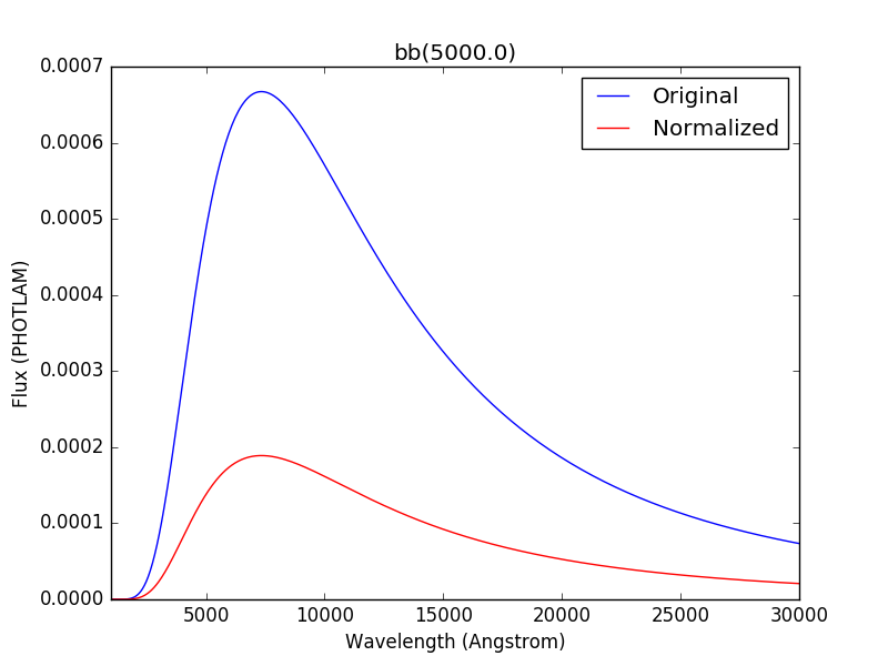
A source spectrum can also be normalized to a given flux value in a given bandpass using its normalize() method. The resultant spectrum is basically the source multiplied with a factor necessary to achieve the desired normalization:

>>> import matplotlib.pyplot as plt  
>>> from synphot import SourceSpectrum, SpectralElement, units
>>> from synphot.models import BlackBodyNorm1D
>>> sp = SourceSpectrum(BlackBodyNorm1D, temperature=5000)
>>> bp = SpectralElement.from_filter('johnson_v')  
>>> vega = SourceSpectrum.from_vega()  # For unit conversion  
>>> sp_norm = sp.normalize(17 * units.VEGAMAG, bp, vegaspec=vega)  
>>> wave = sp.waveset
>>> plt.plot(wave, sp(wave), 'b', wave, sp_norm(wave), 'r')  
>>> plt.xlim(1000, 30000)  
>>> plt.xlabel('Wavelength (Angstrom)')  
>>> plt.ylabel('Flux (PHOTLAM)')  
>>> plt.title(sp.meta['expr'])  
>>> plt.legend(['Original', 'Normalized'], loc='upper right')  

Integration is done with the integrate() method. It can use trapezoid or analytical integration (if the latter is available). The type of integration being done can be controlled with software configuration or keyword. By default, trapezoid integration is done in internal units:

>>> from astropy import units as u
>>> from synphot import SourceSpectrum, units, conf
>>> from synphot.models import GaussianFlux1D
>>> sp = SourceSpectrum(GaussianFlux1D, mean=6000*u.AA, fwhm=10*u.AA,
...                     total_flux=1*(u.erg/(u.cm**2 * u.s)))
>>> sp.integrate()  
<Quantity 3.02046758e+11 ph / (s cm2)>
>>> with conf.set_temp('default_integrator', 'analytical'):
...     print(f'{repr(sp.integrate())}')  
<Quantity 3.02046994e+11 ph / (s cm2)>
>>> sp.integrate(integration_type='analytical')  
<Quantity 3.02046994e+11 ph / (s cm2)>
>>> sp.integrate(flux_unit=units.FLAM)  
<Quantity 0.99999972 erg / (s cm2)>
>>> sp.integrate(flux_unit=units.FLAM, integration_type='analytical')  
<Quantity 1. erg / (s cm2)>

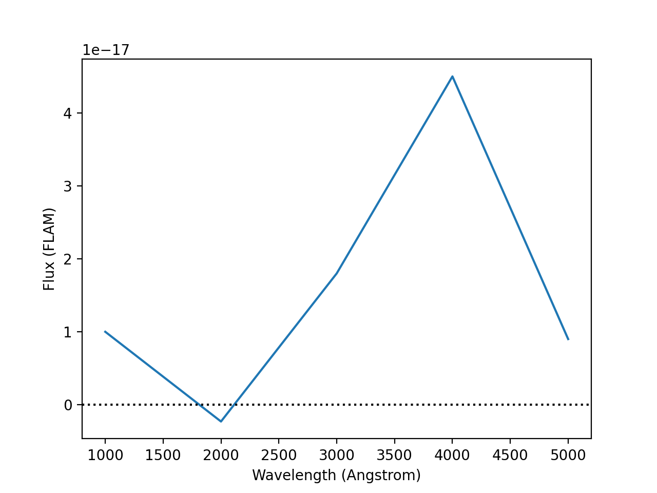
Arrays

Creating source spectrum from arrays is recommended when the input file is in a format that is not supported by synphot. You can read the file however you like using another package and store the wavelength and flux as arrays to be processed by synphot as an empirical model.

The example below creates and plots a source from some given arrays. It also demonstrates that you can choose to keep negative flux values (however unrealistic), if desired:

from synphot import SourceSpectrum, units
from synphot.models import Empirical1D
wave = [1000, 2000, 3000, 4000, 5000]  # Angstrom
flux = [1e-17, -2.3e-18, 1.8e-17, 4.5e-17, 9e-18] * units.FLAM
sp = SourceSpectrum(
    Empirical1D, points=wave, lookup_table=flux, keep_neg=True)
sp.plot(flux_unit=units.FLAM)
plt.axhline(0, color='k', ls=':')

(Source code, png, hires.png, pdf)

Blackbody Radiation

Blackbody radiation is defined by Planck’s law (Rybicki & Lightman 1979):

\[B_{\lambda}(T) = \frac{2 h c^{2} / \lambda^{5}}{\exp(h c / \lambda k T) - 1}\]

where the unit of \(B_{\lambda}(T)\) is \(erg \; s^{-1} cm^{-2} \mathring{A}^{-1} sr^{-1}\) (i.e., FLAM per steradian).

BlackBodyNorm1D generates a blackbody spectrum in PHOTLAM for a given temperature, normalized to a star of 1 solar radius at a distance of 1 kpc. This is to be consistent with ASTROLIB PYSYNPHOT.

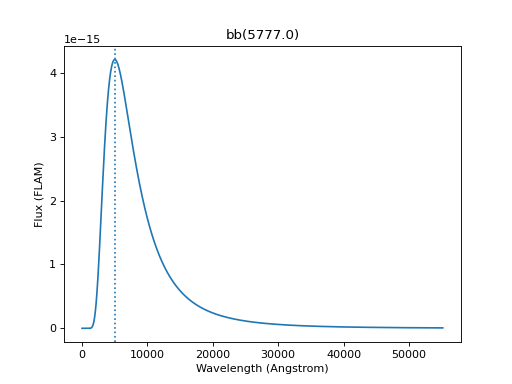
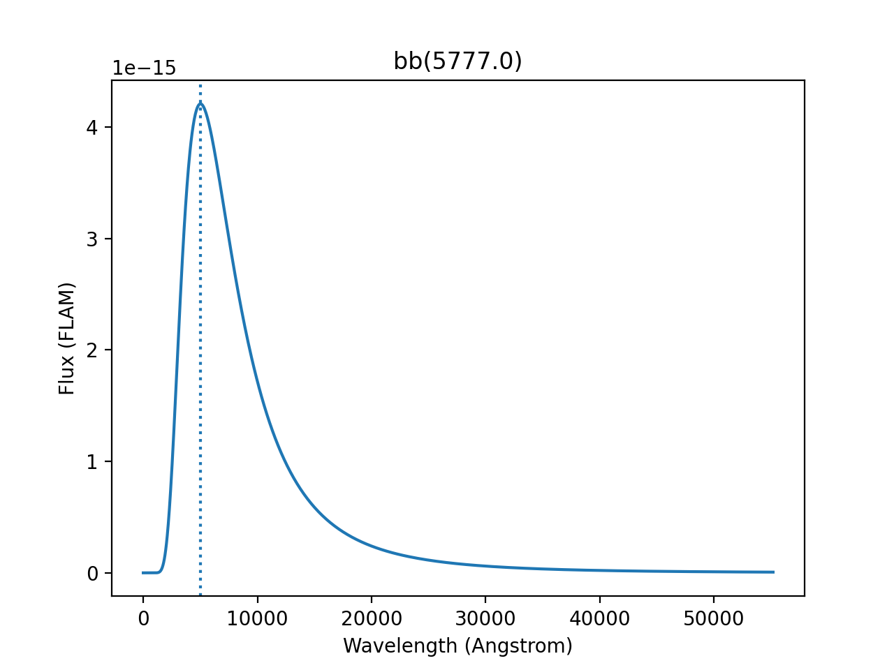
The example below creates and plots a blackbody source at 5777 K:

import matplotlib.pyplot as plt
from synphot import SourceSpectrum
from synphot.models import BlackBodyNorm1D
sp = SourceSpectrum(BlackBodyNorm1D, temperature=5777)
sp.plot(flux_unit='flam', title=sp.meta['expr'])
plt.axvline(sp.model.lambda_max, ls=':')

(Source code, png, hires.png, pdf)

File

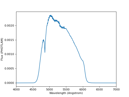
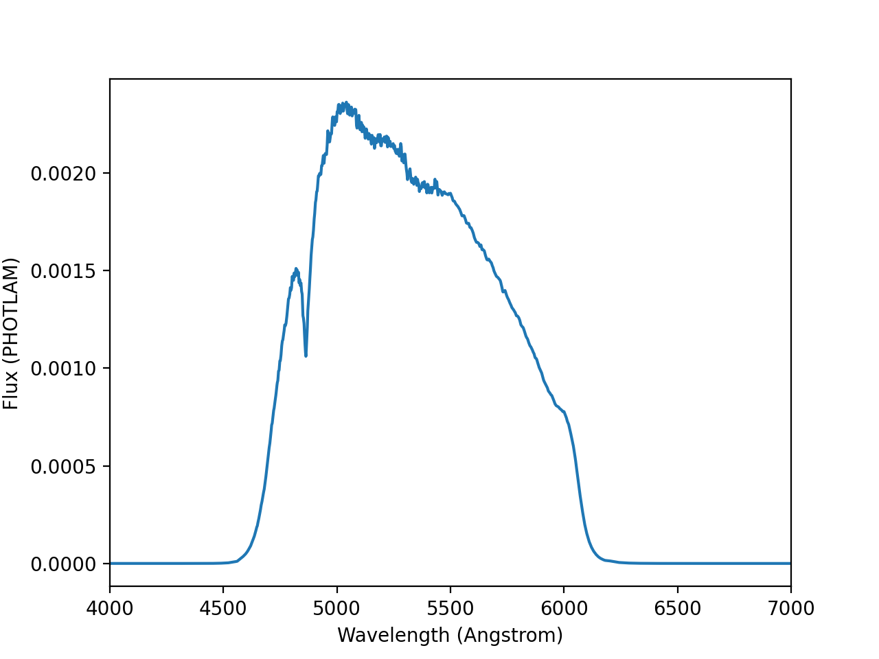
A source spectrum can also be defined using a FITS or ASCII table containing columns of wavelength and flux. See FITS Table Format and ASCII Table Format for details on how to create such tables.

The example below loads and plots a source spectrum from FITS table in the software test data directory:

import os
from astropy.utils.data import get_pkg_data_filename
from synphot import SourceSpectrum
filename = get_pkg_data_filename(
    os.path.join('data', 'hst_acs_hrc_f555w_x_grw70d5824.fits'),
    package='synphot.tests')
sp = SourceSpectrum.from_file(filename)
sp.plot(left=4000, right=7000)

(Source code, png, hires.png, pdf)

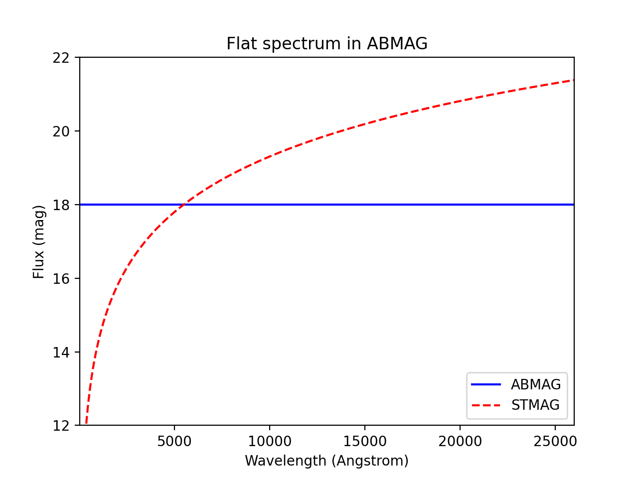
Flat

\[f(x) = A\]

A flat (uniform) spectrum has a constant flux value in the given flux unit, except the following, as per ASTROLIB PYSYNPHOT:

• STMAG - Constant value in the unit of FLAM.

• ABMAG - Constant value in the unit of FNU.

These are currently unsupported:

• count

• OBMAG

Note that flux that is constant in a given unit might not be constant in another (see example below). Such a model has no waveset defined (i.e., no clear wavelength constraints on where the feature of interest lies). Therefore, wavelength values must be explicitly provided for sampling and plotting.

The example below creates and plots a flat source with the amplitude of 18 ABMAG and shows that it is not flat in STMAG:

import matplotlib.pyplot as plt
from astropy import units as u
from synphot import SourceSpectrum
from synphot.models import ConstFlux1D
sp = SourceSpectrum(ConstFlux1D, amplitude=18*u.ABmag)
wave = range(10, 26000, 10)
plt.plot(wave, sp(wave, flux_unit=u.ABmag), 'b',
         wave, sp(wave, flux_unit=u.STmag), 'r--')
plt.xlim(10, 26000)
plt.ylim(12, 22)
plt.ylabel('Flux (mag)')
plt.xlabel('Wavelength (Angstrom)')
plt.title('Flat spectrum in ABMAG')
plt.legend(['ABMAG', 'STMAG'], loc='lower right')

(Source code, png, hires.png, pdf)

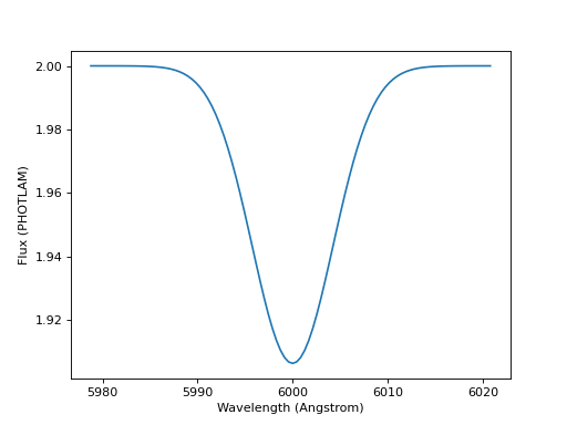
Gaussian Absorption

To create a Gaussian absorption feature, you can first create Gaussian Emission and then subtract it from a continuum (e.g., Flat):

from astropy import units as u
from synphot import SourceSpectrum
from synphot.models import GaussianFlux1D, ConstFlux1D
em = SourceSpectrum(GaussianFlux1D, mean=6000, fwhm=10,
                    total_flux=3.3e-12*u.erg/(u.cm**2 * u.s))
bg = SourceSpectrum(ConstFlux1D, amplitude=2)
sp = bg - em
sp.plot()

(Source code, png, hires.png, pdf)

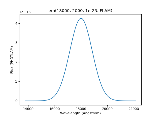
Gaussian Emission

\[ \begin{align}\begin{aligned}f(x) = A \; e^{- \frac{\left(x - x_{0}\right)^{2}}{2 \; \sigma^{2}}}\\\sigma = \frac{\text{FWHM}}{2 \; \sqrt{2 \; \ln 2}}\\A = \frac{f_{\text{tot}}}{\sqrt{2 \; \pi} \; \sigma}\end{aligned}\end{align} \]

where \(f_{\text{tot}}\) is the desired total flux.

GaussianFlux1D generates a Gaussian emission spectrum using input values (central wavelength, FWHM, and total flux) that are somewhat consistent with ASTROLIB PYSYNPHOT.

The example below creates and plots a Gaussian source centered at 1.8 micron with FWHM of 200 nm and the given total flux. As stated in Overview, conversion to internal units happen behind the scenes:

from astropy import units as u
from synphot import SourceSpectrum
from synphot.models import GaussianFlux1D
sp = SourceSpectrum(GaussianFlux1D, mean=1.8*u.micron, fwhm=200*u.nm,
                    total_flux=1e-26*u.W/(u.m**2))
sp.plot(title=sp.meta['expr'])

(Source code, png, hires.png, pdf)

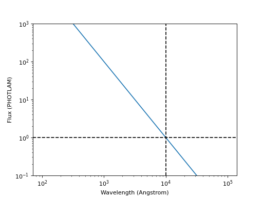
Powerlaw

\[f(x) = A \; (x / x_{0})^{-\alpha}\]

where A should be set to 1 if you want to be consistent with ASTROLIB PYSYNPHOT.

PowerLawFlux1D generates a powerlaw source spectrum. Such a model has no waveset defined (i.e., no clear wavelength constraints on where the feature of interest lies). Therefore, wavelength values must be explicitly provided for sampling and plotting.

The example below creates and plots a powerlaw source with a reference wavelength of 1 micron and an index of -2:

import matplotlib.pyplot as plt
from astropy import units as u
from synphot import SourceSpectrum
from synphot.models import PowerLawFlux1D
sp = SourceSpectrum(PowerLawFlux1D, amplitude=1, x_0=1*u.micron, alpha=2)
wave = range(100, 100000, 50) * u.AA
sp.plot(wavelengths=wave, xlog=True, ylog=True, bottom=0.1, top=1000)
plt.axvline(sp.model.x_0.value, color='k', ls='--')  # Ref wave
plt.axhline(sp.model.amplitude.value, color='k', ls='--')  # Ref flux

(Source code, png, hires.png, pdf)

specutils

A source can be constructed from and written to specutils.Spectrum1D object. See specutils documentation for more information on how to use Spectrum1D.

The example below writes a Gaussian Emission to a Spectrum1D object in the flux unit of Jansky:

>>> from astropy import units as u
>>> from synphot import SourceSpectrum
>>> from synphot.models import GaussianFlux1D
>>> sp = SourceSpectrum(GaussianFlux1D, mean=1.8*u.micron, fwhm=200*u.nm,
...                     total_flux=1e-26*u.W/(u.m**2))
>>> spec = sp.to_spectrum1d(flux_unit=u.Jy)

Meanwhile, this example reads in a source from a Spectrum1D object:

>>> from astropy import units as u
>>> from specutils import Spectrum1D
>>> from synphot import SourceSpectrum
>>> spec = Spectrum1D(spectral_axis=[100, 300]*u.nm, flux=[0.1, 0.8]*u.nJy)
>>> sp = SourceSpectrum.from_spectrum1d(spec)

Thermal

ThermalSpectralElement handles a spectral element with thermal properties, which is important in infrared observations. Its thermal_source() method produces a thermal (blackbody) source spectrum. This is usually not used directly, but rather as part of the calculations for thermal background for some instrument. See stsynphot documentation regarding “thermal background” for more details.

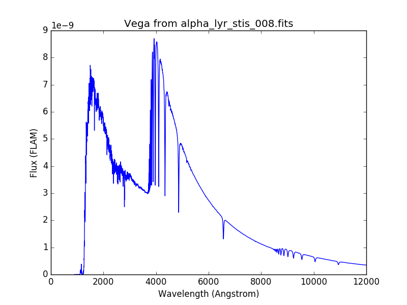
Vega

synphot uses built-in Vega spectrum for VEGAMAG calculations. It is loaded from synphot.conf.vega_file using from_vega().

The example below loads and plots the built-in Vega spectrum:

>>> from synphot import SourceSpectrum
>>> sp = SourceSpectrum.from_vega()  
>>> sp.plot(right=12000, flux_unit='flam', title=sp.meta['expr'])